Formalizing Rubin's theorem

This last semester, I followed Pr. Laurent Bartholdi’s course on computer-assisted proofs in Lean, both because I wanted to get back into the field of computer proofs, and because I was excited at the idea of contributing to Mathlib, which is an impressively large collection of theorems and mathematical tools, all proven in Lean.

About a month into the lecture, Laurent handed me his work-in-progress formalization of Rubin’s theorem, which was still written for Lean 3, with the task to port it to Lean 4 and to make some progress with this formalization. Since then, I have successfully finished this formalization, and I am currently in the process of cleaning it up and slowly getting it merged into Mathlib!

In this blog entry, I will try my best to introduce the necessary knowledge required to understand what Rubin’s theorem is about, and then go into the interesting moments of the process of formalizing this theorem in Lean.

Groups, topologies and group actions

This is a crash course on the necessary concepts of groups, topologies and group actions to be able to formulate Rubin’s theorem, and hopefully develop an intuition for what it means.

These are structures that you most likely have already encountered somewhere, and they have a lot of interesting and useful properties besides the elementary ones listed here.

If you are already familiar with these concepts, then you can safely jump to the last section of this chapter.

Groups

Groups are a common structure that arises when studying objects like addition, multiplication, matrices or sequences of moves on a Rubik’s cubes. All four of these examples have a binary operation that can be cancelled out or “undone”, yielding a “do nothing” element (respectively $0$, $1$, the identity matrix and the empty sequence).

A group mirrors these properties in a more abstract and generic way, allowing us to forget about the specifics of how each of the examples above work. As such, every group is made up of four components, each mirroring one of the interesting aspects of these structures:

• The carrier set,

  which we will refer to as $\mathbf{G}$. It contains all of the elements of the structure we wish to study.

• An identity element,

  here written $1$ (or $1_{G}$). It represents the “do nothing” element.

• A binary operation,

  here represented using the multiplication symbol $*$. It represents the act of combining or chaining together two elements $g$ and $h$ to get a compound element $g * h$, that does what $h$ does followed by what $g$ does.

  Note: the left-to-right interpretation is also possible, but I will use the right-to-left interpretation, since this is how matrices naturally multiply together.

• The inverse operation,

  which is often written $g^{-1}$. It represents the act of “undoing” an element. For instance, the Rubik’s cube move $R^{-1}$ (also written $R'$) undoes the move $R$.

Then, these four components follow a couple of rules:

• Identity:

  Multiplying by $1_{G}$ must do nothing, so for any $g \in \mathbf{G}$, we have $1 * g = g$ and $g * 1 = g$.

• Associativity:

  For any $g, h, i \in \mathbf{G}$, we have $g * (h * i) = (g * h) * i$. This essentially lets us forget about parentheses.

• Inverse:

  For each element $g \in \mathbf{G}$, multiplying it by $g^{-1}$ cancels it out: $g * g^{-1} = 1$ and $g^{-1} * g = 1$.

• Closure:

  If $g$ and $h$ are in $\mathbf{G}$, then $g * h$ and $g^{-1}$ are also in $\mathbf{G}$

There are many examples of groups in the wild, some of which you might already be familiar with. For instance:

• Integers, armed with addition: $\mathbf{G} = \mathbb{Z}$, $1_{G} = 0$, $g *_{G} h = g + h$ and $g^{-1} = -g$
• Non-zero rational numbers, armed with multiplication: $\mathbf{G} = \mathbb{Q} \setminus {0}$, $1_{G} = 1$, $g *_{G} h = g * h$ and $g^{-1} = 1/g$
• Invertible, square matrices
• Sequences of moves on a Rubik’s cube, with $*$ representing the chaining of two sequences of moves, and $M^{-1}$ undoing all of the moves in $M$

I highly recommend watching 3Blue1Brown’s video on group theory for a more visual introduction to group theory, and Lingua Mathematica’s video on the associativity rule for a more intuitive interpretation of the group axioms.

Note that multiplication doesn’t need to commute: for any two elements $g$ and $h$, $g * h \ne h * g$ is allowed.
This is notably the case for matrix multiplication, or on a Rubik’s cube (see example below). In fact, we will see later that groups in which multiplication always commutes (also known as abelian groups) cannot be used in Rubin’s theorem.

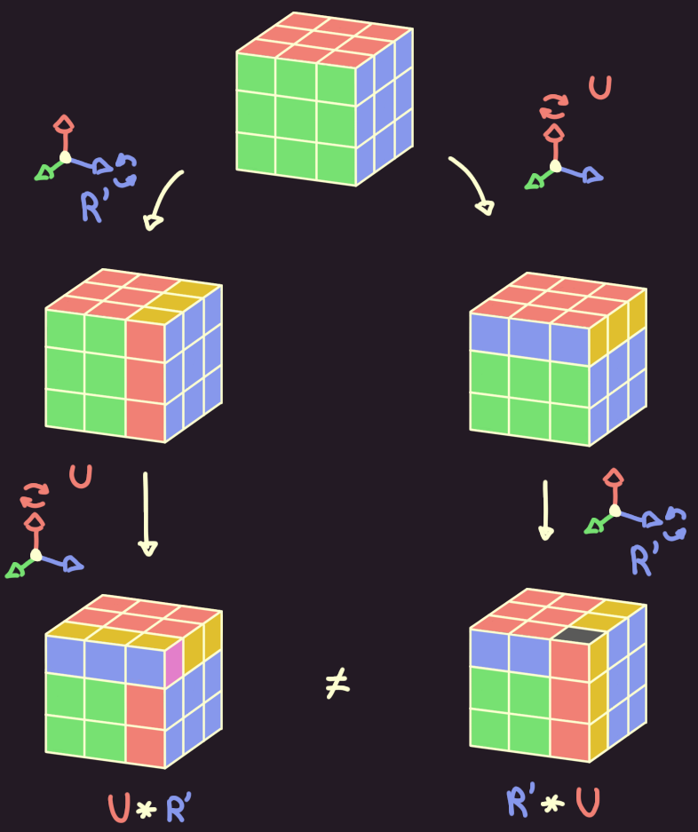On a Rubik’s cube, when doing U after R' (ie. U*R'), we get a different position than when doing R' after U (ie. R'*U).

Lastly a subgroup of $\mathbf{G}$ is a subset $\mathbf{H}$ of $\mathbf{G}$ containing $1_{G}$, and in which the multiplication and inverse operations are closed: $\forall g \in \mathbf{H}, g^{-1} \in \mathbf{H}$ and $\forall g, h \in \mathbf{H}, g * h \in \mathbf{H}$.

The subgroups of $\mathbf{G}$ can be ordered with the $⊆$ relationship, and there are two subgroups found in every group:

• $\mathbf{G}$ itself, which is the biggest subgroup of $\mathbf{G}$, and is therefore usually referred to as the top subgroup, or $\top$
• $\{1_{G}\}$, which only contains $\mathbf{G}$’s identity element $1_{G}$. This is the smallest possible subgroup of $\mathbf{G}$, so it is also referred to as the bottom subgroup, or $\bot$

Topological spaces

You might remember from calculus the concept of a continuous function: it is a function which takes as input a real number, and outputs another real number, such that you never have to “lift your pen” to draw the graph of this function.

However, this “pen”-based definition quickly falls short when we consider continuity for other kinds of functions:

• What does it mean for a function to be continuous on the rational numbers $\mathbb{Q}$? The “pen” always has to “jump” from one rational to the other, but that shouldn’t be a reason to discard the function $f(x) = x^2$ as discontinuous.
• For functions that take as input two numbers instead of one, the “pen” would need to draw surfaces instead of lines, which is something that pens are usually incapable of doing.
• What about functions that operate on other functions? Translating a function (for instance, $\phi(f) = (x \mapsto f(x) + 1)$) sounds like a continuous operation, but I doubt I would convince anyone if I said that I never lifted my “function pen” while doing so.

“Can you tell where I lifted my function pen?”

To remedy this, mathematicians came up with the concept of a topological space. Like groups, a topological space is made up of a few basic building blocks, which follow a set of rules:

• A set $\mathbf{X}$, called the universe.
• A collection of subsets of $\mathbf{X}$, referred to as $\tau$ or the open sets of $\mathbf{X}$.
• The empty set must be in $\tau$: $\empty \in \tau$.
• $\mathbf{X}$ itself must be in $\tau$: $\mathbf{X} \in \tau$.
• If $S$ and $T$ are both open, then their intersection must also be open: $S \in \tau \Rightarrow T \in \tau \Rightarrow S \cap T \in \tau$.
• If we have a collection of open sets $\mathbf{C}$ (such that $\forall S \in \mathbf{C}, S \in \tau$), then the union of all of these sets must be open.
• A set $S$ is closed if $\mathbf{X} \setminus S$ is open.

In the case of the real numbers, $\tau(\mathbb{R})$ contains all of the open intervals, and unions of open intervals.
$(0, 1)$ and $(-\infty, 0)$ are both open sets, but $(0, 1]$ and $[2, 2] = \{2\}$ aren’t.
In fact, $\{2\}$ is closed, since $\mathbb{R} \setminus \{2\} = (-\infty, 2) ∪ (2, +\infty)$ is open.

Using this definition, a function $f$ is then said to be continuous if for every open set $S \in \tau$, the set of points that $f$ maps inside of $S$ must also be open: $f^{-1}(S) \in \tau$. For functions from $\mathbb{R}$ to $\mathbb{R}$, this condition is equivalent to the pen-based definition.

The function $f$ is discontinuous, because for $S = (2, 3) \in \tau$, $f^{-1}(S) = [2, 3)$ isn’t open.

Conditions on topological spaces

You might have noticed that the above definition for a topological space leaves a lot of freedom on the choice of $\tau$, perhaps even too much freedom.
On the one hand, if $\tau = \{\empty, \mathbf{X}\}$ (the trivial topology of $\mathbf{X}$), then the only open sets are the universe and the empty set, which is not very useful.
On the other hand, if $\tau = \{S \;|\; S \subseteq \mathbf{X}\}$ (the discrete topology of $\mathbf{X}$), then all the sets are open (and coincidentally closed), so every function from $\mathbf{X}$ is continuous.

For this reason, we often impose some common, additional conditions that $\tau$ and $\mathbf{X}$ must respect. Here are the ones that Rubin’s theorem requires:

$\mathbf{X}$ must be Hausdorff: for any two $x \ne y$, you can find an open set $S$ around $x$ and an open set $T$ around $y$, that do not intersect ($S \cap T = \empty$).

For the reals, assuming that $x < y$, the sets $S = (-\infty, \frac{x + y}{2})$ and $T = (\frac{x + y}{2}, +\infty)$ satisfy this condition. A similar construction can be done for $x > y$.

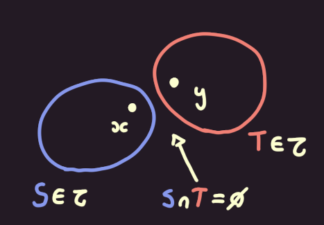If $\mathbf{X}$ is Hausdorff, then no matter how close $x$ and $y$ are, we can draw disjoint open sets around both of them.

$\mathbf{X}$ must not have any isolated points: for every $x \in X$, the set that only contains it, $\{x\}$, must not be open. This condition essentially forbids us from choosing the discrete topology.

We saw before that for the reals, $\{x\} = [x, x]$ is never an open set (it is instead only a closed set), so $\mathbb{R}$ has no isolated points.

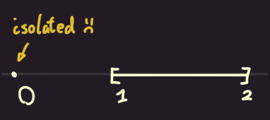In the topological space $\mathbb{R} \cap (\{0\} \cup [1, 2])$, the point $0$ is isolated.

$\mathbf{X}$ must be locally compact: for every point $x \in X$, it should be possible to obtain a compact set in the neighborhood of $x$; that is, there is a set $T$ such that every sequence of points in $T$ must converge to a point in $T$, and there exists a set $S \in \tau$ such that $x \in S$ and $S ⊆ T$.

The reals are an example of a locally compact space, since every closed set is compact (for instance, any sequence in $[0, 1]$ cannot converge to any number outside of that range). We thus simply have to take the interval $T = [x - 1, x + 1]$ to obtain a compact set in the neighborhood of some $x$, and $S = (x - 1/2, x + 1/2)$.

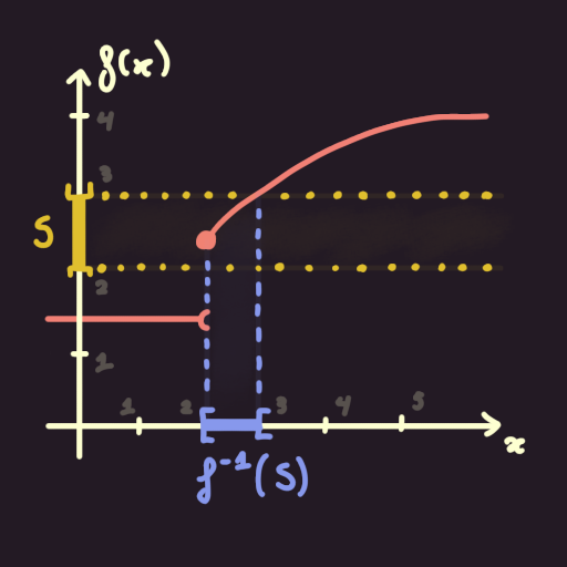
Interior and closure

There are two common operations in topology that allows one to obtain an open or a closed set from any arbitrary set $S$:

• The interior of $S$ is the largest open subset of $S$: $int(S) \subseteq S$ and $\forall T \in \tau, T \subseteq S \Rightarrow T \subseteq int(S)$. It can be obtained by taking the union of all open subsets of $S$.
• The closure of $S$ is the smallest closed superset of $S$, it is the dual of the interior operation: $cl(S) = X \setminus int(X \setminus S)$

Note that the interior of $S$ may be empty if $S$ is too small, and the closure of $S$ can be $\mathbf{X}$ itself if $S$ is too big.

Group actions

A group $\mathbf{G}$ is said to acts on some set $\mathbf{X}$ if, for every $x \in \mathbf{X}$:

• For every $g \in \mathbf{G}$, the result of the action of $g$ on $x$ (which we write $g \bullet x$) is in $\mathbf{X}$: $g \bullet x \in \mathbf{X}$
• For every $g \in \mathbf{G}$ and $h \in \mathbf{G}$, the action of $g * h$ corresponds to the compound action of $h$ and $g$: $(g * h) \bullet x = g \bullet (h \bullet x)$
• The action of $1$ does not move $x$: $1 \bullet x = x$

An example of such a group action is the matrix-vector multiplication: when evaluating $(M_1 * M_2) \bullet v$, we can first transform $v$ by $M_2$ and then transform it by $M_1$, or we can compute $M = M_1 * M_2$ once and then transform $v$ by $M$.

Another famous example of a group action is the action of the cyclic group by rotating points on a 2D plane:

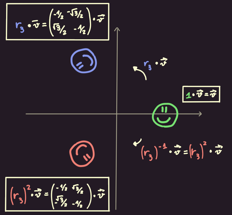The group action of $(r_3)^i \bullet x$ corresponds to rotating $x$ by $120 * i$ degrees.

Conditions on group actions

Just like with topological spaces, Rubin’s theorem requires that the group action respects a few additional rules, namely:

The action must be faithful: for any $g, h \in \mathbf{G}$, if $g$ and $h$ move points in the same fashion, then they are equal: $(\forall x, g \bullet x = h \bullet x) \Rightarrow g = h$.
In other words, we can tell group elements apart simply by looking at how they move points in space.

The action must be continuous: for every $g \in \mathbf{G}$, the function $f(x) = g \bullet x$ must be continuous.

The action must be locally dense: this is a somewhat complex condition that is specific to Rubin’s theorem, but it can be summarized as follows:

• Pick an open set $S \in \tau$ and some $x \in S$.
• Find all the elements $g \in \mathbf{G}$ that leave points outside of $S$ unmoved ($\forall y \not\in S, g \bullet y = y$); the set of all of these elements forms a subgroup of $\mathbf{G}$, which we will call $H$.
• Construct $H \bullet x = \{ h \bullet x \;|\; h \in H \}$, the set of all the points towards which $x$ gets moved by the elements of $H$.
• Compute the closure of that set: $cl(H \bullet x)$.
• Then, there must exist an open set $T$ containing $x$ that is a subset of the previously-constructed set: $x \in T \in \tau$ and $T \subseteq cl(H \bullet x)$.

Essentially, this last condition requires that for arbitrarily small open sets $S$, we must always find enough elements in $\mathbf{G}$ to “fill in” enough of the space in $S$ around $x$.

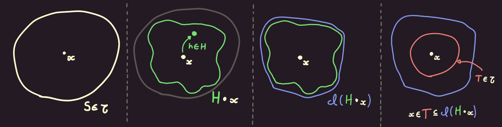A visual representation of the condition that an action is locally dense.

Homeomorphism

A homeomorphism is a function $f : \mathbf{X} \rightarrow \mathbf{Y}$ such that:

• $f$ is bijective: it maps one-to-one values in $\mathbf{X}$ to values in $\mathbf{Y}$
• $f$ is continuous
• $f^{-1}$ is also continuous

Homeomorphisms are useful tools, since the open sets in $Y$ can be obtained from the open sets in $X$ by mapping them through $f$, and vice-versa ($\tau(\mathbf{Y}) = f(\tau(\mathbf{X}))$ and $\tau(\mathbf{X}) = f^{-1}(\tau(\mathbf{Y}))$).
As such, if one can construct a homeomorphism between two topological spaces, then these two spaces will share a lot properties and be essentially topologically equivalent.

Rubin’s theorem

We can now finally state Rubin’s theorem!

An action of a group $\mathbf{G}$ on a topological space $\mathbf{X}$ is called a Rubin action if:

• $\mathbf{X}$ is Hausdorff, has no isolated points and is locally compact (see Conditions on topological spaces above for a refresher).
• The action of $\mathbf{G}$ on $\mathbf{X}$ is faithful, continuous and locally dense (see Conditions on group actions).

Then, if we have two Rubin actions of $\mathbf{G}$ on $\mathbf{X}$ and of $\mathbf{G}$ on $\mathbf{Y}$, then there exists a homeomorphism $\phi : \mathbf{X} \rightarrow \mathbf{Y}$ that preserves the action of $\mathbf{G}$: $g \bullet \phi(x) = \phi(g \bullet x)$.

The existence of this homeomorphism means that the two spaces and their respective group action by $\mathbf{G}$ are essentially unique: we can losslessly go from one to the other.

Computer-assisted theorem proving

Computer theorem provers are programs that provide ways to express and verify mathematical theorems. The advantage of using such a theorem prover is that you reduce human error in the proof verification process to almost zero: as long as the theorem prover functions well, and your definitions are accurate, you can be guaranteed that your proof is 100% correct if the theorem prover accepts it.

The one downside when one wants to prove things using such a theorem prover, though, is that one has to prove these mathematical statements to a computer. No taking shortcuts, hand-waving details away or leaving lemmas as exercise to the reader; everything needs to be proven thoroughly, from properties as simple as 1 + 1 = 2 to the Fundamental Theorem of Algebra.

Theorem provers have been around for a few decades now, notably with Coq and Isabelle.

Lean is, in comparison, a relatively recent addition to the theorem prover landscape, as it was first released in 2013. Its main selling point is that it is easier to use (it provides a VSCode extension whose quality is on-par with rust-analyzer’s), and it powers the community-developped library, Mathlib, which aims to formalize as much of modern mathematics as possible.

While not being a central theorem, Laurent and I believe that Rubin’s theorem would be a neat addition to Mathlib, as it can be used as a stepping stone in a few already-existing theorems (J. Belk et al. have compiled a nice list of its applications in their article).

Our proof closely follows the proof by J. Belk et al, as it is the most concise proof of this theorem to date. However, as I started working on this project, all I had was a link to the paper and a 1000-lines long, unfinished proof, written for Lean 3, covering the first few lemmas of the paper. So, there was and still is a lot left to do to get to this project’s final goal.

Porting to Lean 4

The first official release of version 4 of Lean was only made a couple of months ago, but projects like Mathlib had been preparing themselves for the release and had already ported themselves over to the newer version. This meant that my first order of business was to port the existing proof over to Lean 4.